The lasso is a modified regression method that gained popularity following the work of Tibshirani (Tibishirani et. al, 1996). It shares similarities with linear regression in that it aims to minimize the difference between observed responses and the predictions of a linear model. However, it sets itself apart by performing variable selection, effectively picking the most important predictors from the available set.
In contrast to linear regression, where all variables receive non-zero coefficients, the lasso offers a solution when there is a large number of irrelevant variables that do not significantly influence the outcome. For example, when predicting GDP based on numerous socio-economic factors, variables like per-capita income may correlate with GDP, while others like healthy life expectancy may not. When many such irrelevant variables exist, including all of them in a linear regression model can be inefficient. The lasso addresses this by constraining the sum of the absolute values of coefficients to be lower (achieving this through a loss function that combines sum of squared errors and the sum of L1 norms of coefficients). This effectively reduces some coefficients, making them zero, and eliminates the corresponding variables from the linear model.
In this article, we will apply the lasso method to a dataset of socio-economic indicators (all from the year 2017 unless specified otherwise) from sources such as the World Bank and the International Monetary Fund. Our goal is to predict GDP using these indicators as predictor variables. Some of these indicators are known to be highly correlated with GDP, while others are not. We will examine whether the lasso eliminates these less relevant variables to achieve sparsity.
Additionally, we aim to explore whether these socio-economic factors can be used to predict the World Happiness Index. This index, inspired by a similar one in Bhutan, was developed by Harvard University academics and is based on global surveys conducted to assess happiness levels.
Downloading the relevant data
Some world bank development indicators
Initially, we will retrieve essential indicators from the World Bank using the WDI (World Development Indicators) package in R. Numerous online resources provide guidance on locating and downloading relevant indicators. You can refer to this tutorial for detailed instructions: https://worldpoliticsdatalab.org/tutorials/data-wrangling-and-graphing-world-bank-data-in-r-with-the-wdi-package/
#WDI::languages_supported()
#WDIsearch('gdp')[1:10,]

dat = WDI(indicator=c("NY.GDP.MKTP.CD",# gdp -# the gross domestic product
                    "SP.DYN.LE00.IN", ## Life expectancy at birth (For all)
                    "SP.DYN.LE00.MA.IN", # Life expectancy at birth (For males)
                    "SP.DYN.LE00.FE.IN", # Life expectancy at birth (For females)
                    "EN.ATM.CO2E.PC", # Co2 emission in metric tonne
                    "NY.GDP.PCAP.KD", # Per capita income
                    "SP.POP.TOTL", # Population size ## in thousands
                    "FP.CPI.TOTL.ZG", # Inflation_consumer_prices ## percentage
                    "SP.DYN.CDRT.IN", # Mortality_rate ## for every 1000
                    "SP.DYN.IMRT.IN", # Infant_mortality_rate ## for every thousand births
                    "EG.ELC.ACCS.ZS"), # access_to_electricity ## percent of the pop.
                  start=2017, end=2017)
Human development index data
The file was manually downloaded from the website ( [https://hdr.undp.org/data-center] (https://hdr.undp.org/data-center)) and the development indices for 2017 and 2018 were extracted and saved in a separate file.
dat_dev_ind <- read_csv("human_development_index_2017_18.csv")
dat_dev_ind
World happiness index
World happiness index for 2018 is downloaded from world happiness report 2018 website [https://worldhappiness.report/ed/2018/] (https://worldhappiness.report/ed/2018/) .
dat_hap_ind <- read_excel("happiness_index.xlsx")
I have also downloaded data from IMF (International Monetary Fund) on some more economic factors, which are stored in separate csv files. We will download them into R dataframe in our local workspace.
d2g <- read_excel("debt_2_gdp.xlsx")
prcap <- read_excel("private_cap_data.xlsx")
pucap <- read_excel("public_cap_data.xlsx")
sub <- read_excel("subsidies_data.xlsx")
tax <- read_excel("taxRevenue_data.xlsx")

d2g <- subset(d2g, select=-c(...1))
colnames(d2g) <- c("debt_2_gdp", "iso2c")
prcap <- subset(prcap, select=-c(...1))
pucap <- subset(pucap, select=-c(...1))
sub <- subset(sub, select=-c(...1))
colnames(sub) <- c("iso2c", "subsidies")
tax <- subset(tax, select=-c(...1))
colnames(tax) <- c("iso2c", "tax_revenue")
Helper file from countrycode package
Our next step involves merging all these individual datasets into a unified one. While we can perform this merging based on country names, a more efficient approach is to use either the ISO-3/ISO-2 codes or IMF codes (from the International Monetary Fund). We can conveniently access these codes for all countries using the ‘countrycode’ library.
dat_with_hap <- dat %>% inner_join(dat_hap_ind, by="iso3c")
dat_hap_dev <- dat_with_hap %>% inner_join(dat_dev_ind, by="iso3c")
library(countrycode)
data(codelist)
country_set <- codelist
country_set <- country_set %>%
  select(country.name.en, iso2c, iso3c, imf, continent, region) %>% filter(!is.na(imf) & !is.na(iso2c))

prcap$imf <- as.numeric(prcap$imf)
pr_dat <- country_set %>% inner_join(prcap, by="imf")
pucap$imf <- as.numeric(pucap$imf)
prNpu_dat <- pr_dat %>% inner_join(pucap, by="imf")
prNpuDe_dat <- prNpu_dat %>% inner_join(d2g, by="iso2c")

final_dat <- dat_hap_dev %>% inner_join(prNpuDe_dat, by="iso2c")
final_dat <- subset(final_dat, select=-c( country.name.en,iso3c.y, country.y, country.x))
colnames(final_dat)
Giving some readable column names to the new dataframe
colnames(final_dat) <- c("iso2c",
                         "iso3c",
                         "year",
                         "gdp",
                         "life_exp_at_birth",
                         "life_exp_at_birth_male",
                         "life_exp_at_birth_female",
                         "co2_emi",
                         "income_per_capita",
                         "population_size",
                         "inflation_consumer_prices",
                         "mortality_rate",
                         "infant_mortality_rate",
                         "access_electricity",
                         "happiness_index",
                         "country",
                         "hdi_2017",
                         "hdi_2018",
                         "imf",
                         "continent",
                         "region",
                         "privCap_2_gdp",
                         "publCap_2_gdp",
                         "debt_2_gdp")
Instead of relying solely on the Gini coefficient for the year 2017, we have opted to use the median Gini coefficient for each country over multiple years. This approach helps address the issue of missing values, which is prevalent when restricting our analysis to a single year, such as 2017.
# fifth_dat <- na.omit(fifth_dat) #
#fifth_dat

sa_da <- WDI(indicator = c("SI.POV.GINI"))

give_gini = function(iso_code){
sa_ve <- unique(sa_da[sa_da$iso3c==iso_code,]$SI.POV.GINI)
return(median(sa_ve[!is.na(sa_ve)]))
}

l_iso3 <- final_dat$iso3c
l_gini <- sapply(l_iso3, give_gini)

final_dat$gini_coefficient <- l_gini


final_dat_numeric <- final_dat %>% select(gdp, life_exp_at_birth, life_exp_at_birth_male, life_exp_at_birth_female, co2_emi, income_per_capita, population_size, inflation_consumer_prices, mortality_rate, infant_mortality_rate, access_electricity,happiness_index,hdi_2017,hdi_2018, gini_coefficient, privCap_2_gdp, publCap_2_gdp, debt_2_gdp)
We will employ the ‘mice’ package to impute missing values, specifically utilizing the lasso method provided by the ‘mice’ package for this purpose.
library(mice)
#md.pattern(final_dat_numeric)
final_dat_complete <- complete(mice(final_dat_numeric, method="lasso.norm"))
Using GDP as a response variable
response <- "gdp"
predictors <- c("life_exp_at_birth",
                "life_exp_at_birth_male",
                "life_exp_at_birth_female",
                "co2_emi",
                "income_per_capita",
                "population_size",
                "inflation_consumer_prices",
                "mortality_rate",
                "infant_mortality_rate",
                "access_electricity",
                "happiness_index",
                "hdi_2017",
                "hdi_2018",
                "gini_coefficient",
                "privCap_2_gdp",
                "publCap_2_gdp",
                "debt_2_gdp")

predictors_plt <- c("gdp","life_exp_at_birth", "life_exp_at_birth_male", "life_exp_at_birth_female", "co2_emi", "income_per_capita", "population_size", "inflation_consumer_prices","mortality_rate","infant_mortality_rate","access_electricity","happiness_index","hdi_2017","hdi_2018", "privCap_2_gdp", "publCap_2_gdp", "debt_2_gdp")
#fifth_dat[,response]
x_plt <- data.matrix(final_dat_complete[,predictors_plt])
Plotting the correlation matrix with histogram and scatterplots
library(corrplot)
M = cor(x_plt)
corrplot(M, method='color', order='alphabet')#+
#labs(title="Color plot of the Correlation matrix of all the variables")
# library("PerformanceAnalytics") #
# chart.Correlation(x_plt, histogram=TRUE, pch=19) #

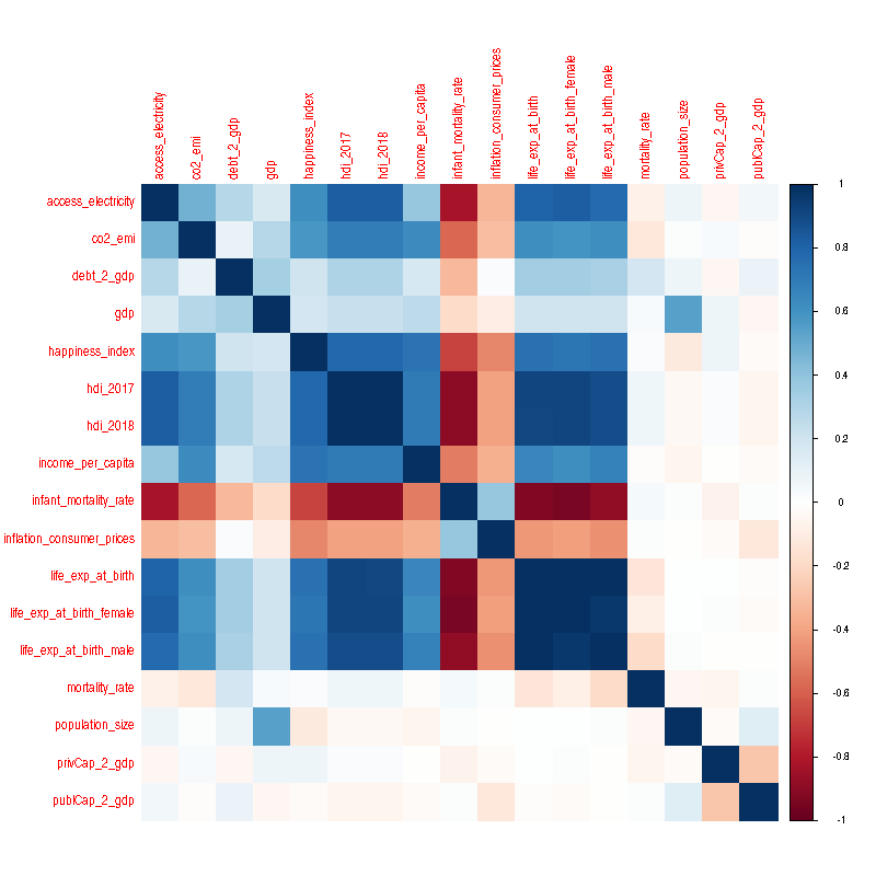
Fig.1. Correlation matrix of all the variables. Gross Domestic Product (GDP) shows high positive correlation with population size while happiness index shows high positive correlation with variables like access_electricity, human development indices (hdi_2017 and hdi_2018), and life expectancies
standardize = function(x){

  z <- (x-mean(x))/sd(x)
  return(z)
  }

set.seed(4)
train <- sample(1:nrow(x), ceiling(2*nrow(x)/3))
test <- (-train)


blacksheep = function(x){

  as.numeric(x)
  }

final_dat_stand <- apply(final_dat_complete, 2, blacksheep)
#final_dat_stand <- as.data.frame(scale(final_dat_stand))

dat_train <- final_dat_stand[train,]
dat_test <- final_dat_stand[test,]
dat_train <- as.data.frame(scale(dat_train))
dat_test <- as.data.frame(scale(dat_train))

x <- apply(x, 2, standardize)
y <- standardize(y)

lm_fit <- lm(gdp~., data=final_dat_stand)


#lasso_pred <- sapply(seq_along(cv.out$lambda), function(i){predict(lasso_fit, s=cv.out$lambda[i], newx = x_test)})
#l_err <- apply(lasso_pred, 2, function(x){sum((x-y_test)^2)})
#plot(ln(grid),l_err)
Splitting the data into training and test batch and fitting the lasso
library(glmnet)
standardize = function(x){

  z <- (x-mean(x))/sd(x)
  return(z)
  }

library(SciViews)
x <- data.matrix(final_dat_complete[,predictors])
y <- data.matrix(final_dat_complete[,response])

set.seed(4)

train <- sample(1:nrow(x), ceiling(2*nrow(x)/3))
test <- (-train)

x_train <- x[train,]
y_train <- y[train]
x_train <- apply(x_train, 2, standardize)
y_train <- standardize(y_train)

x_test <- x[test,]
y_test <- y[test]

x_test <- apply(x_test, 2, standardize)
y_test <- standardize(y_test)

x <- apply(x, 2, standardize)
y <- standardize(y)

#lasso_fit <- glmnet(x[train, ], y[train], alpha=1) ## alpha=1 --> the lasso, alpha=0 --> ridge regression, 0<alpha<1 --> elastic net

lasso_fit <- glmnet(x_train, y_train, alpha=1)
#set.seed(1)
cv.out <- cv.glmnet(x_train, y_train, alpha=1)
plot(cv.out)

bestlam <- cv.out$lambda.min
# lasso_pred <- predict(lasso_fit, s=bestlam, newx = x_test) #
# mean((lasso_pred - y_test)^2) #
#  #
grid <- cv.out$lambda
out <- glmnet(x_train, y_train, alpha=1, lambda = grid)
lasso_coef <- predict(out, type = "coefficients", s=bestlam)


#lasso_pred <- sapply(seq_along(cv.out$lambda), function(i){predict(lasso_fit, s=cv.out$lambda[i], newx = x_test)})
#l_err <- apply(lasso_pred, 2, function(x){sum((x-y_test)^2)})
#plot(ln(grid),l_err)

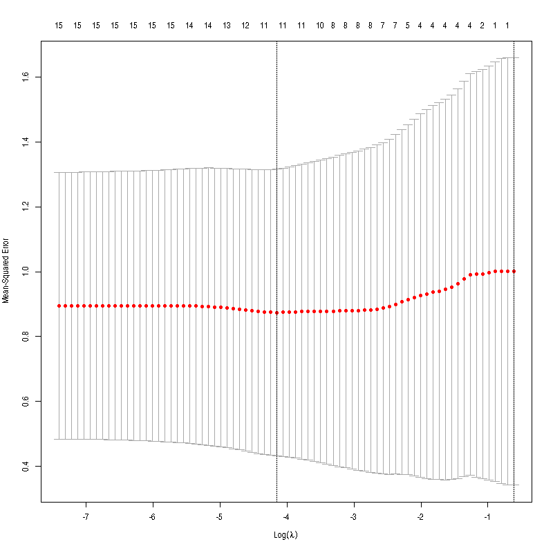
Fig.2. We plotted the Average Mean Squared Errors (MSEs) against the tuning parameter, which controlled the extent of the sparsity constraint within the loss function, during the bootstrapping procedure. The vertical bars, straddling individual data points, represent the standard deviation of the errors.
lasso_coef_df <- as.data.frame(matrix(lasso_coef))
lasso_coef_df$predictors <- rownames(lasso_coef)
colnames(lasso_coef_df) <- c("size_of_the_coefficients", "predictors")


p <- ggplot(lasso_coef_df, aes(x=predictors, y=size_of_the_coefficients)) + geom_col(width=0.5)
p + coord_flip()#+
  #labs(title="Important variables (with non-zero coefficients)",
  #subtitle="Response: GDP")

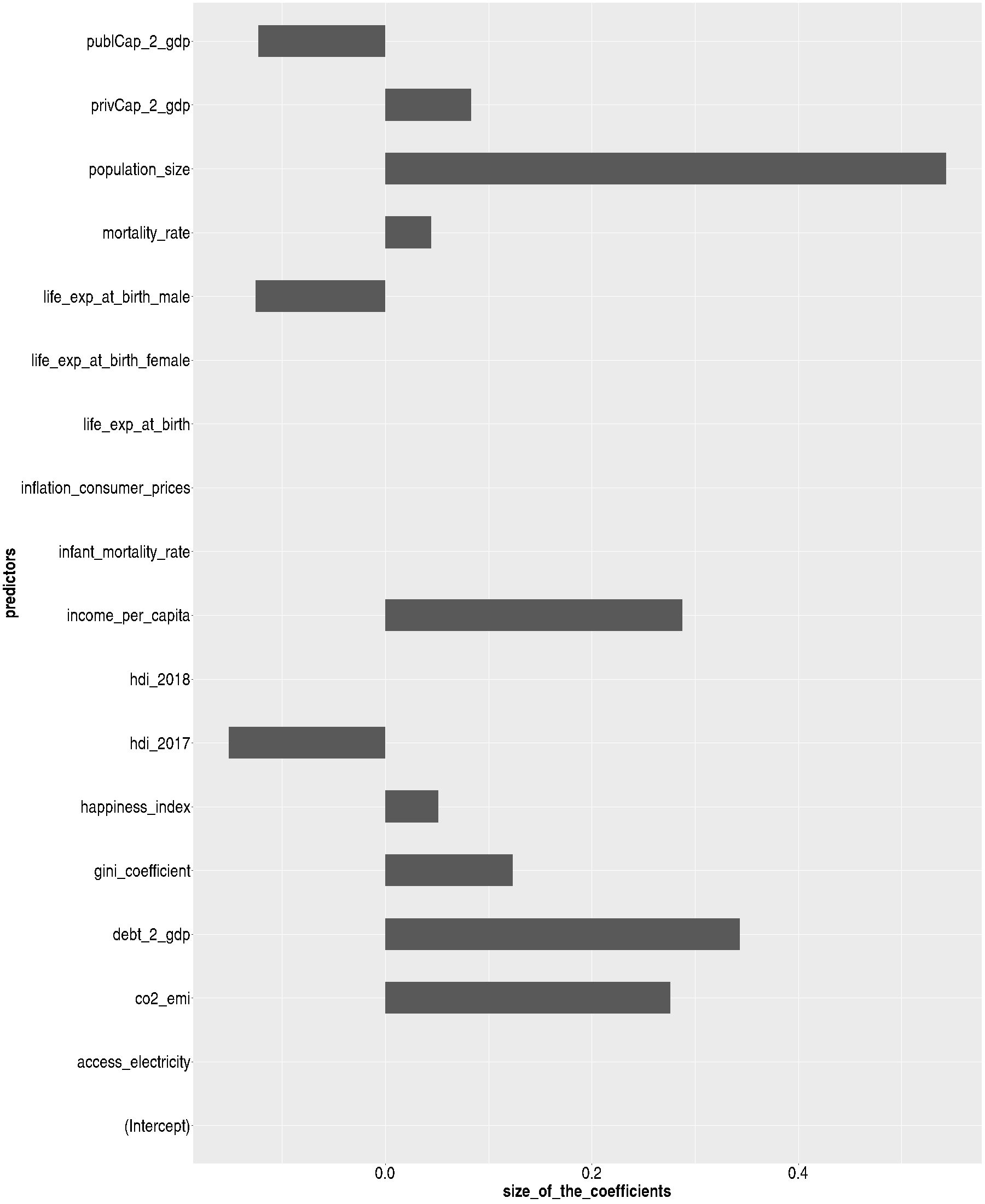
Fig.3. In the linear model with GDP as the response variable and the minimum cross-validation error, the coefficients of significant variables are retained. Conversely, the lasso method introduces additional sparsity constraints, reducing the coefficients of other variables to zero.
Happiness Index as the response variable
response <- "happiness_index"
predictors <- c("gdp",
                "life_exp_at_birth",
                "life_exp_at_birth_male",
                "life_exp_at_birth_female",
                "co2_emi",
                "income_per_capita",
                "population_size",
                "inflation_consumer_prices",
                "mortality_rate",
                "infant_mortality_rate",
                "access_electricity",
                "hdi_2017",
                "hdi_2018",
                "gini_coefficient",
                "privCap_2_gdp",
                "publCap_2_gdp",
                "debt_2_gdp")
Splitting the data into training and test batch and fitting the lasso - for happiness
library(glmnet)
standardize = function(x){

  z <- (x-mean(x))/sd(x)
  return(z)
}

library(SciViews)
x <- data.matrix(final_dat_complete[,predictors])
y <- data.matrix(final_dat_complete[,response])

set.seed(4)

train <- sample(1:nrow(x), ceiling(2*nrow(x)/3))
test <- (-train)

x_train <- x[train,]
y_train <- y[train]
x_train <- apply(x_train, 2, standardize)
y_train <- standardize(y_train)

x_test <- x[test,]
y_test <- y[test]

x_test <- apply(x_test, 2, standardize)
y_test <- standardize(y_test)

x <- apply(x, 2, standardize)
y <- standardize(y)

#lasso_fit <- glmnet(x[train, ], y[train], alpha=1) ## alpha=1 --> the lasso, alpha=0 --> ridge regression, 0<alpha<1 --> elastic net

lasso_fit <- glmnet(x_train, y_train, alpha=0)
#set.seed(1)
cv.out <- cv.glmnet(x_train, y_train, alpha=0)
plot(cv.out)

bestlam <- cv.out$lambda.min
# lasso_pred <- predict(lasso_fit, s=bestlam, newx = x_test) #
# mean((lasso_pred - y_test)^2) #
#  #
grid <- cv.out$lambda
out <- glmnet(x_train, y_train, alpha=0,lambda = grid)
lasso_coef <- predict(out, type = "coefficients", s=bestlam)


#lasso_pred <- sapply(seq_along(cv.out$lambda), function(i){predict(lasso_fit, s=cv.out$lambda[i], newx = x_test)})
#l_err <- apply(lasso_pred, 2, function(x){sum((x-y_test)^2)})
#plot(ln(grid),l_err)
lasso_coef_df <- as.data.frame(matrix(lasso_coef))
lasso_coef_df$predictors <- rownames(lasso_coef)
colnames(lasso_coef_df) <- c("size_of_the_coefficients", "predictors")


p <- ggplot(lasso_coef_df, aes(x=predictors, y=size_of_the_coefficients)) + geom_col(width=0.5)
p + coord_flip()

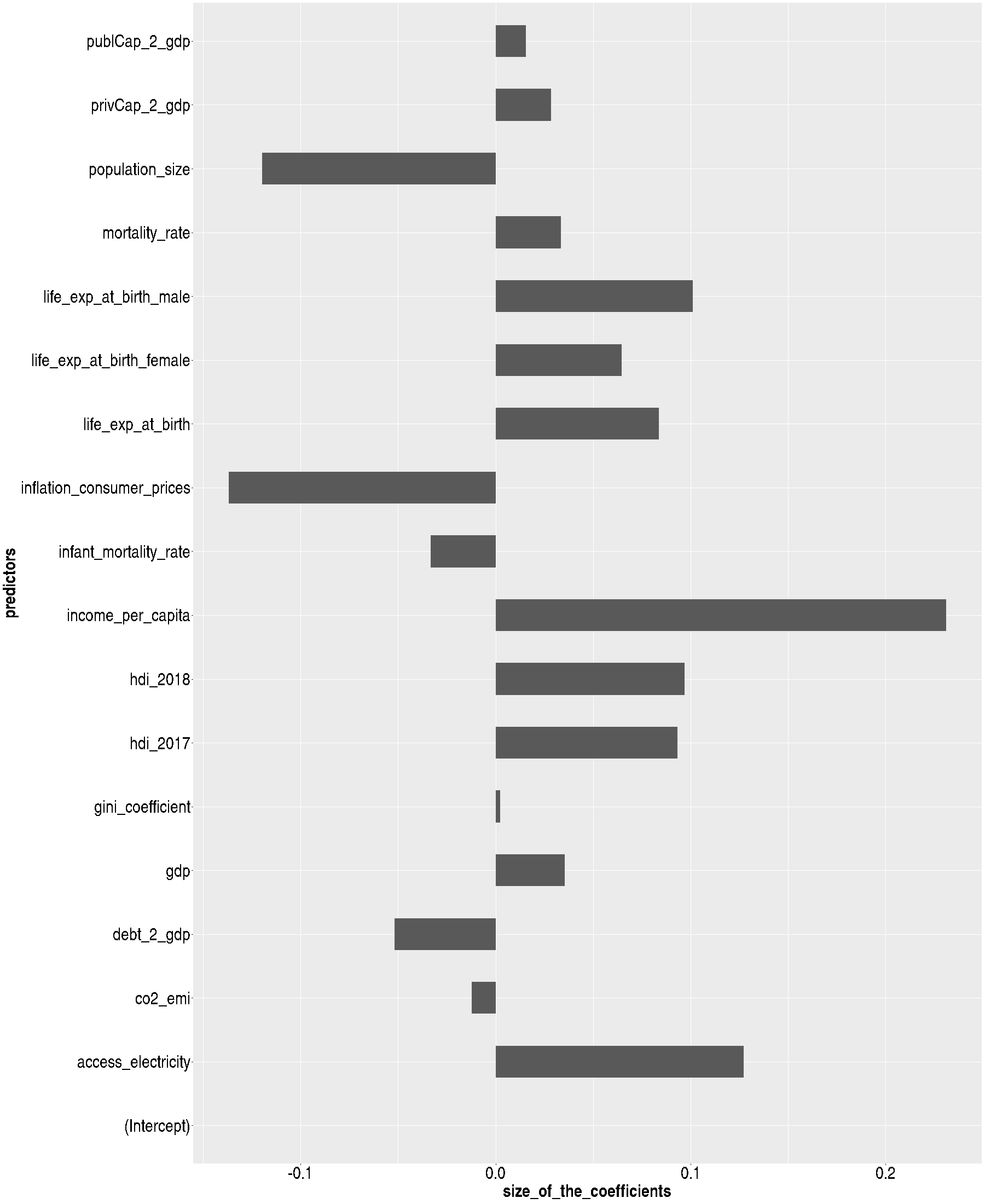
Fig.4. The coefficients of the important variables in the linear model (with the minimum cross-validation error) with Happiness Index as the response variable. Notice new predictors that predict happiness index (like access to electricity ) and some opposite trends (like population size).